Project 05
Data & Signal
Two pieces of work where the deliverable was a decision, not a model: one on how many labels a survey actually needs to pay for, and one on pulling a planted signal back out of noise.
Galaxy morphology — label-efficient transfer learning
17,736 real survey images · ResNet50 · Galaxy10-DECaLS
I fine-tuned a ResNet50 on 17,736 real images from the Dark Energy Camera Legacy Survey, labelled by the Galaxy Zoo citizen-science campaign, across ten morphological classes.
1 receipt
- galaxy-morphology-transferMethod, splits, hyperparameters and full results.
I chose macro-F1 as the primary metric rather than accuracy, because the classes are imbalanced and accuracy would have flattered the model on the common ones. I trained with class-weighted loss and stopped on validation macro-F1.
1 receipt
- READMEMetric choice stated with the reason; AdamW, ReduceLROnPlateau, early stopping.
Then I ran the same experiment at 1%, 5%, 10% and 100% of the labels, evaluating all four on the identical held-out test set — because the question I actually wanted answered was not "how good can this get" but "how few labels do we need to pay for".
1 receipt
- READMEStratified subsets, one shared test set, four measured points.
The most interesting result was an error analysis, not a score: the smallest class scored perfect recall while a mid-sized one scored worst. Distinctiveness beats frequency — so annotation budget should go to the ambiguous classes, not the rare ones.
1 receipt
- READMEPer-class recall — Cigar-shaped Smooth 100.00% on 334 training examples; Disturbed 59.26%.
Hover any point
How many labels do you actually need?
~709 images · 5% of the set
75.31% accuracy
The jump that matters: +22 points of accuracy for one afternoon of expert labelling. After this, the curve flattens.
accuracymacro-F1ResNet50 · Galaxy10-DECaLS · 17,736 labelled survey images
The findingFive per cent of the labels — about 709 images, one afternoon of expert work — gets you to 75.3% accuracy. Ten per cent gets you 78.1%. That second doubling costs the same again and buys under three points. If I were advising someone paying for annotation, that is the entire recommendation, and it is worth more than the 87.3% I got from labelling everything.
Honest note: the training code for this one is not published yet — the repository currently holds the write-up and the results. It is on my machine and it is going up.
Two detection pipelines, and one I am not showing you
Simulation study — signal injection and recovery
I wanted to know whether a method could find a thing it had not been told the location of. So for each of three problems I generated a catalogue, planted a known signal inside it, and then measured how much of that signal the detector got back. Two of the three are below. The third fitted a value for dark energy that is not physically possible, which means the pipeline is wrong somewhere I have not found yet — so it is not on this page, and that is the only honest place for it to be. None of these use real observational data, and I would not present them as if they did — the whole point of injection-recovery is that you know the right answer in advance and can therefore grade the method honestly.
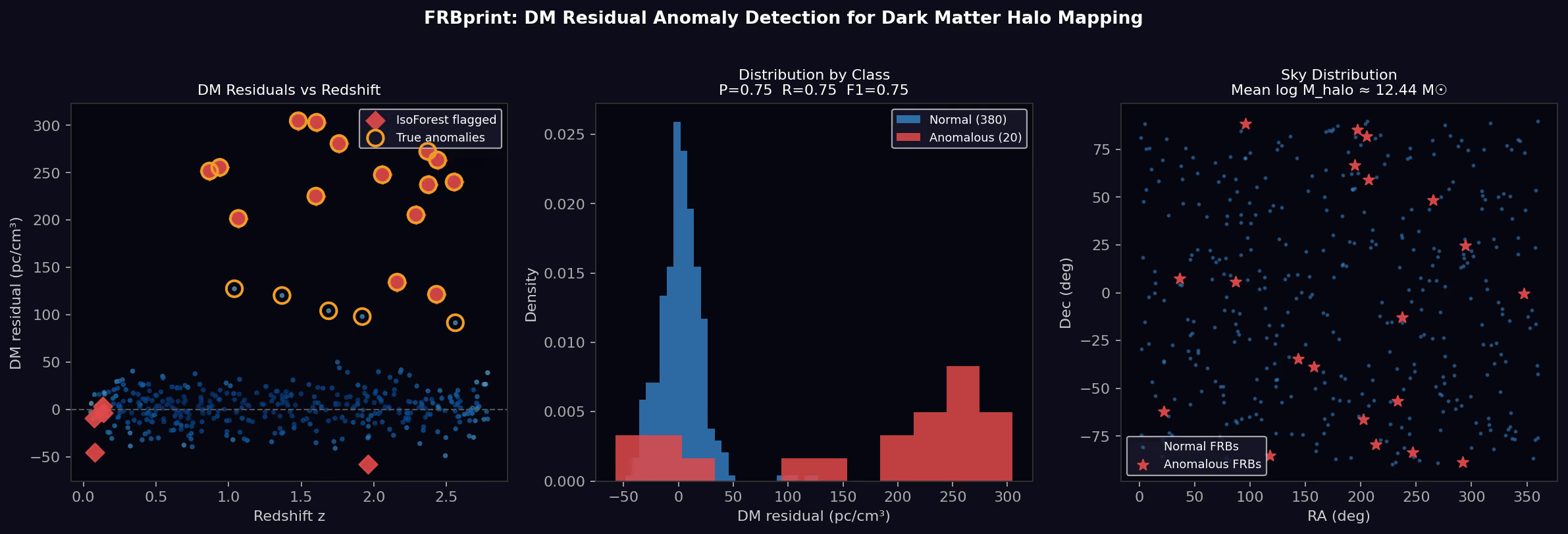
1 receipt
- frbprintMethod, the injected catalogue, and the full confusion matrix.
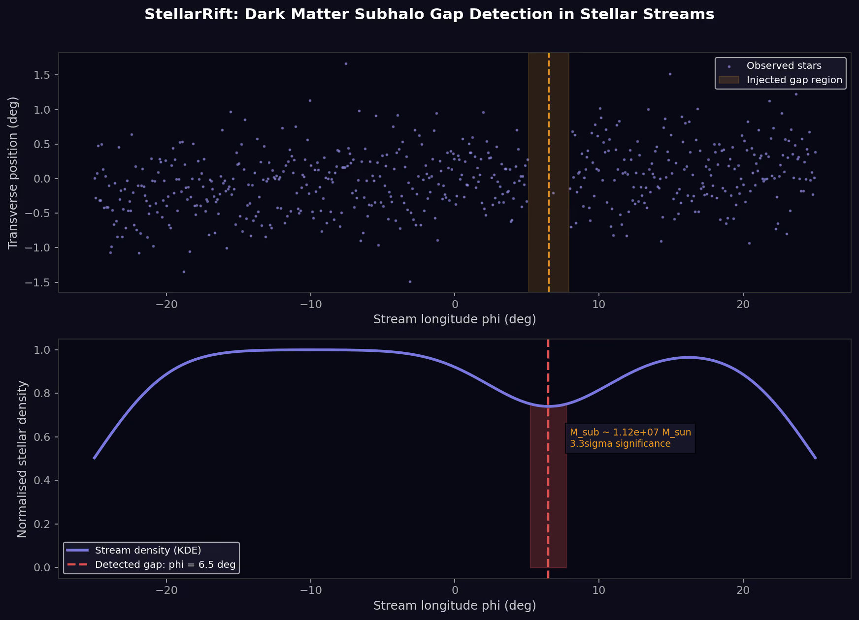
1 receipt
- stellarriftThe KDE detector and the injected gap position.
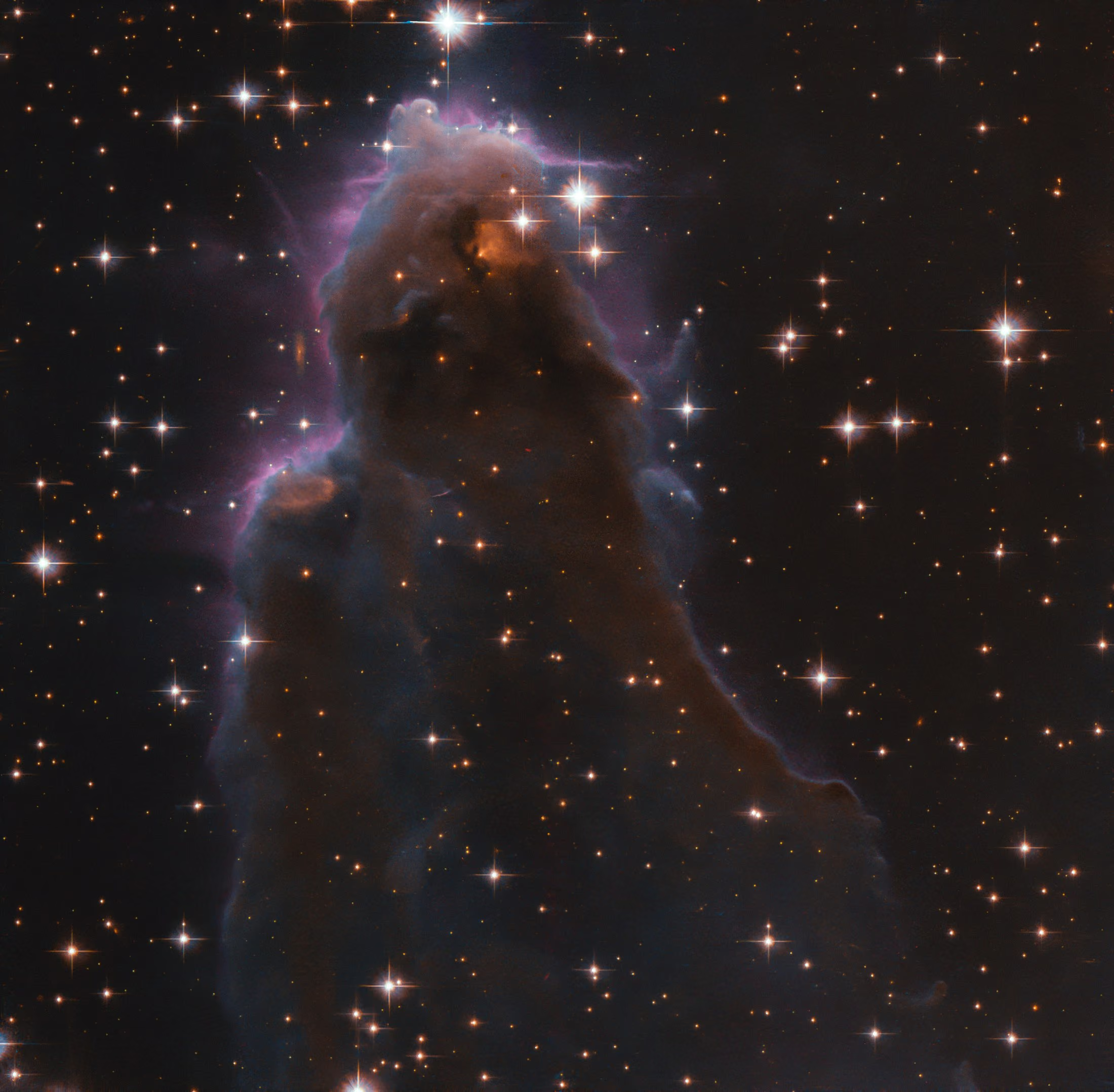
frEGGs, in the Cygnus region
Dense knots that survive precisely because they were dense enough to.
Radiation from nearby giant stars blasts away the loose gas around them, and only the densest clumps hold together — each one now forming a star inside. What survives the measurement is not what was most common. It is what was most robust.
A frEGGs-plosion of star formation · NASA, ESA and the Hubble Heritage Team (STScI/AURA) · CC BY 4.0